
This guide shows how to perform bearing capacity calculations in Python using Eurocode 7, with transparent and auditable workflows for geotechnical engineers.
Bearing capacity is one of the most fundamental calculations in geotechnical engineering. You have probably done it many times in Excel or inside a proprietary design tool. So why don’t we try to do it again in Python?
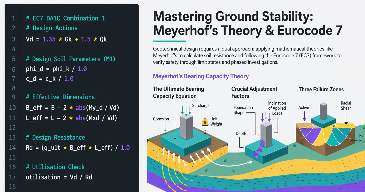
When you run a bearing capacity calculation inside a spreadsheet, the formula chain is invisible. A reviewer cannot see which version of the Nq expression you used or check whether your shape factors account for load inclination. Python changes that, as every assumption is a variable with a name, and every intermediate result is printed with a structured log at the end, documenting exactly what was assumed and why.
This post shows how to go from Eurocode 7 design logic to structured Python code, in a way that is:
- Defensible (you can stand behind it in a design review)
- Auditable (clear assumptions and traceability)
- Reusable (not a one-off spreadsheet)
Automate Bearing Capacity Checks (EC7)
Eurocode 7 adopts the classical Terzaghi-Meyerhof form of the bearing capacity equation, extended with correction factors for shape, load inclination, and foundation depth.
Before writing a single line of code, we need to step back and fully understand the engineering problem we are trying to automate and all variables involved.
Bearing capacity in Eurocode 7 is not just a formula, but a combination of soil behaviour, loading conditions, geometry effects, and design philosophy. That means it is important to identify:
- All the variables involved (soil parameters, foundation dimensions, load components, groundwater conditions);
- How they interact (e.g. how moments translate into eccentricity and reduce the effective area); and
- The sequence of calculations required (from bearing capacity factors to correction factors and finally resistance checks under different design approaches)
The list below shows all the inputs we need to produce the calculation for the drained condition based on φ’ and c’:
- Foundation geometry inputs:
- Foundation geometry (shape and geometry)
- Loading (vertical actions, horizontal actions and moments)
- Groundwater
- Ground Properties inputs:
- Drained parameters (φ’ and c’)
- Undrained parameters (Su)
- Unit weights (bulk and effective)
- Overburden at foundation level
- Design Approach – In this case, we will use DA-1 Combination 1 from EC7.
Drained Analysis — EC7 Annex D
Based on Section 6.5.2 in EC7 Part 1, the design value of the actions (Vd) should be equal to or lower than the design value of the resistance to the actions (Rd) both in the short and long term, depending on the ground.
In Annex D, a sample analytical method for bearing resistance calculation is defined as informative:
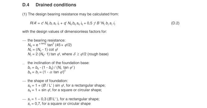
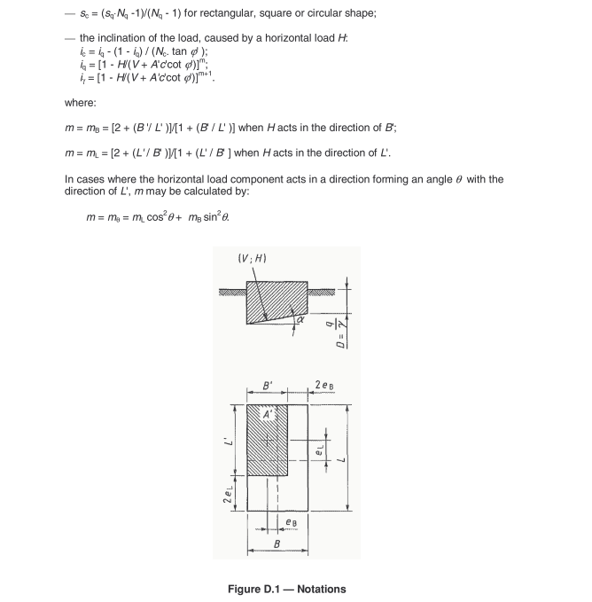
Figure D.1 — EN 1997-1:2004 Eurocode 7: Geotechnical Design – Part 1: General Rules, Annex D (informative): Sample analytical method for bearing resistance calculation
Translating Engineering into Code Variables
Assumptions to state before the code:
- Drained analysis only, using phi’ and c’.
- EC7 Annex D style analytical method adopted.
- Single equivalent founding stratum.
- Effective area method used for eccentric loading.
- Horizontal load inclination factors included.
- Base inclination, ground slope, and nearby slope factors excluded.
- Partial factors for design Approach DA1 – Combination 1:
- Actions (Set A1):
- Unfavourable permanent: γG = 1.35
- Variable: γQ = 1.5
- Soil parameters (Set M1):
- gamma_phi = 1.0
- gamma_c = 1.0
- Resistance factor (Set R1):
- gamma_R = 1.0 (UK NA typical for spread foundations)
- Actions (Set A1):
Step 1 – Foundation, Soil and Actions to DA1C1
To start easily, we will define the problem with variables:
import math

# -----------------------------
# 1. INPUTS
# -----------------------------

# Characteristic soil parameters (drained)
phi_k_deg = 34.0      # characteristic friction angle (degrees)
c_k = 0.0             # characteristic effective cohesion (kPa)
gamma_eff = 19.0      # effective unit weight (kN/m3)

# Foundation geometry
B = 10.0      # footing width (m)
L = 10.0      # footing length (m)
Df = 0.0      # embedment depth (m)

# Characteristic actions
Gk = 3000.0           # permanent vertical action (kN)
Qk = 500.0            # variable vertical action (kN)
Hx_k = 0.0            # characteristic horizontal load in x (kN)
Hy_k = 0.0            # characteristic horizontal load in y (kN)
Mx_k = 0.0            # moment about x-axis (kNm)
My_k = 0.0            # moment about y-axis (kNm)

# -----------------------------
# 2. DA1C1 PARTIAL FACTORS
# -----------------------------
gamma_G = 1.35
gamma_Q = 1.50
gamma_phi = 1.0
gamma_c = 1.0
gamma_R = 1.0

# Design actions
Vd = gamma_G * Gk + gamma_Q * Qk
Hxd = gamma_G * Hx_k
Hyd = gamma_G * Hy_k
Mxd = gamma_G * Mx_k
Myd = gamma_G * My_k

# Design soil parameters (M1)
phi_d_deg = phi_k_deg / gamma_phi
c_d = c_k / gamma_c
phi_d = math.radians(phi_d_deg)

# -----------------------------
# 3. EFFECTIVE DIMENSIONS
# -----------------------------
eB = Myd / Vd if Vd != 0 else 0.0
eL = Mxd / Vd if Vd != 0 else 0.0

B_eff = B - 2.0 * abs(eB)
L_eff = L - 2.0 * abs(eL)

if B_eff <= 0 or L_eff <= 0:
    raise ValueError("Effective footing dimensions are zero or negative.")
Step 2 – Bearing Capacity Factors
This is a major audit risk point, so make sure you give the sources and assumptions (e.g. Vesic / Meyerhof / EC7 preference)
# -----------------------------
# 4. BEARING CAPACITY FACTORS
# -----------------------------
Nq = math.exp(math.pi * math.tan(phi_d)) * math.tan(math.pi / 4 + phi_d / 2) ** 2
Nc = (Nq - 1.0) / math.tan(phi_d)
Ngamma = 2.0 * (Nq - 1.0) * math.tan(phi_d)

# -----------------------------
# 5. CORRECTION FACTORS
# -----------------------------
# Shape factors
sq = 1.0 + (B_eff / L_eff) * math.sin(phi_d)
sc = (sq * Nq - 1.0) / (Nq - 1.0)
sgamma = 1.0 - 0.3 * (B_eff / L_eff)

# -----------------------------
# 6. INCLINATION FACTORS
# -----------------------------
Hd = math.hypot(Hxd, Hyd)
load_ratio = min(Hd / Vd, 0.99)

iq = (1.0 - load_ratio) ** 2
igamma = (1.0 - load_ratio) ** 2
ic = iq - (1.0 - iq) / max(Nc * math.tan(phi_d), 1e-9)
Step 3 – Overburden
# -----------------------------
# 7. OVERBURDEN
# -----------------------------
q = gamma * Df
Step 4 – Bearing Capacity Calculation
# -----------------------------
# 8. DESIGN RESISTANCE
# -----------------------------

q_ult = (
    c_d * Nc * sc * ic * dc
    + q_eff * Nq * sq * iq * dq
    + 0.5 * gamma_eff * B_eff * Ngamma * sgamma * igamma * dgamma
)

Rd = (q_ult * B_eff * L_eff) / gamma_R   # kN

utilisation = Vd / Rd
Step 5 – Result logging for Auditability
# -----------------------------
# 7. STRUCTURED OUTPUT
# -----------------------------
results = {
    "Design approach": "EC7 DA1 Combination 1",
    "Vd_kN": Vd,
    "Rd_kN": Rd,
    "utilisation": utilisation,
    "phi_d_deg": phi_d_deg,
    "c_d_kPa": c_d,
    "B_eff_m": B_eff,
    "L_eff_m": L_eff,
    "Nq": Nq,
    "Nc": Nc,
    "Ngamma": Ngamma,
    "q_ult_kPa": q_ult,
}

for key, value in results.items():
    print(f"{key}: {value}")
You can also download the full code from GitHub: bearing-capacity-check-drainedEC7
What this example shows is that coding a bearing capacity check is not about translating an equation into Python. It is about structuring engineering logic in a way that is transparent, traceable, and reviewable. Every assumption, from the choice of bearing capacity factors to how eccentricity is treated, is explicitly written into the calculation.
This is where Python becomes more powerful than spreadsheets: not because it is faster, but because it forces clarity. In the next step, this framework can be extended to include Eurocode 7 Design Approaches (DA1C1 and DA1C2), partial factors, and sensitivity analyses to understand how uncertainty in parameters such as φ’ propagates into design capacity.
Always consider that automation does not replace professional judgement, and you must clearly state assumptions, limitations and validation steps.